Research Note
A Dual-View Normalization–Chunking Stage for Vietnamese Mathematical Documents
June 19, 2026 · Harry Tran
Download formal paper hereAbstract
Vietnamese mathematics textbooks reach document processing pipelines as text streams in which a single problem span is composed of a statement, a set of answer choices, a worked solution, and a terminal answer, all interleaved with dense mathematical markup. Generic document partitioners handle these structures poorly. Splitting on surface cues such as blank lines shreds logical problem units into fragments, whereas embedding the raw text allows repeating mathematical control sequences to dominate the semantic representation, burying the prose signals that mark topic transitions. Removing formulas before embedding addresses the representation problem but destroys the mathematical content that subsequent parser stages require to build question-answer records. This paper presents a dual-view architecture that resolves this representation conflict. The algorithm applies a mathematical normalizer to construct a simplified, placeholder-based view of the document to drive semantic embedding and structural tagging, while maintaining a parallel, original-text view to reconstruct the final chunks. A validation guard monitors the output assembly and aborts writing if any placeholder leaks into the delivered text. In evaluations across six documents containing 12,937 paragraph blocks and 46,732 mathematical tokens, the coupled architecture preserves 100% of mathematical tokens, whereas a normalization-only baseline preserves only 0.03%. On a structural boundary-placement metric, the normalized representation does not improve boundary accuracy, scoring 0.39 compared to 0.43 for chunking on raw text. Normalization functions as an embedding-safety mechanism that protects mathematical content for downstream parsing, rather than a method for improving boundary placement.
1. Introduction
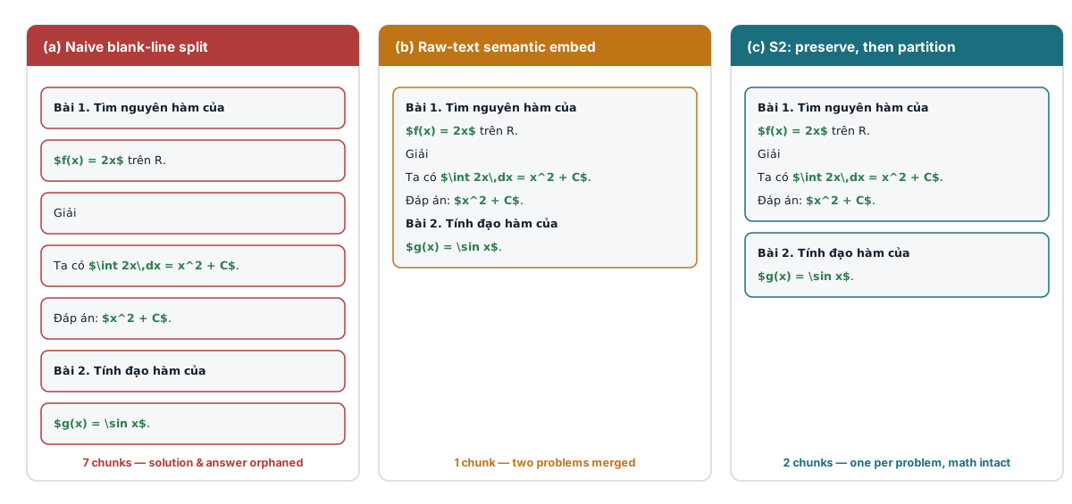
A problem unit in a Vietnamese mathematics textbook is a compound object structured around a regular grammar. The unit opens with a distinct structural marker, such as a question or example label, and contains multiple subcomponents including multiple-choice options, a worked solution, and a terminal answer. The primary task of a document segmenter is to partition the document stream such that each logical unit remains whole. Two distinct error modes break this structure: splitting a single problem across multiple chunks, which orphans solutions and answers, and merging adjacent problems into a single chunk, which fuses separate exercises.
Standard semantic chunking methods determine segment boundaries by placing cuts where the embedding signal shifts. In mathematical textbooks, this approach is compromised because mathematical formula tokens dominate the embedding space. Repeating mathematical markup structures, such as fractions and summations, recur across unrelated exercises, inflating the cosine similarity between adjacent blocks. As a result, distinct problems appear semantically similar to the text encoder, and the boundaries between them are obscured. The failure is representational: the mathematical syntax dominates the prose signal before any boundary decision is made.
To address this representation issue, mathematical markup can be isolated from the text. Replacing each formula with a typed placeholder removes the recurring formula confound, enabling the text encoder to focus on the semantic prose. While this preprocessing step improves embedding cleanliness, it destroys the content. Downstream parsing stages that convert chunks into database records depend on the original mathematical formulas. Normalization that benefits the text encoder rendering the text unusable for subsequent extraction. Quantitative measurements establish this cost: a baseline that normalizes the document without a restoration step preserves only 0.03% of the source mathematical tokens in its output.
The algorithm described in this paper maintains two parallel representations of the document. Each paragraph-level block retains a normalized view, which drives semantic embedding, spectral clustering, and structural tagging, and an original view, which is used to construct the final output. The two views are aligned line by line during preprocessing. Document partitioning is computed on the normalized view, while the output chunks are assembled from the original view. A validation guard aborts the assembly if a placeholder leaks into the delivered text. This dual-view contract enables a mathematical normalizer to run for the benefit of the text encoder while ensuring that no mathematical notation is lost in the final output.
The experiments establish a specific boundary for this architecture. The coupled segmenter combines document partitioning with mathematical preservation, serving as the only evaluated configuration that partitions the document without losing mathematical syntax. However, on boundary placement accuracy, normalization does not improve performance. The coupled segmenter scores lower than both the raw-text chunking baseline and the naive normalization baseline, a difference that is consistent across all six test documents and statistically significant. The primary role of normalization in this pipeline is to protect the embedding space and ensure downstream usability, rather than to improve boundary placement.
2. Problem Setting: Re-Evaluating Vietnamese Math Document Segmentation
The target of the segmentation process is the individual problem unit, defined by its structural grammar. Each unit begins with an opener, such as a question or example label, and may contain multiple-choice options, a worked solution, and a terminal answer line. A correct segment contains exactly one such unit from the opener to the final answer. Cutting a solution or answer away from its opener orphans content that depends on the question context, while merging two openers into a single chunk fuses independent problems, corrupting downstream extraction.
The document input contains three interacting sources of noise. First, digitizing documents yields varying block granularities. Digitized documents contain approximately 40% more paragraph blocks, more frequent line breaks, and higher delimiter noise than native digital documents. Second, Vietnamese diacritics and mathematical symbols share the same Unicode byte stream, requiring the segmenter to process prose and markup simultaneously. Third, documents contain page-level artifacts, including running headers, figure labels, table boilerplate, and character misreads where section symbols are transcribed as mathematical dollar signs. These sources compound: digitized pages yield more blocks, each containing more delimiter artifacts, amidst a mix of Unicode prose and mathematical markup.
Naive segmentation strategies fail in systematic ways. Fixed token-length splitting ignores document layout, cutting mid-problem when the token budget is exhausted. Blank-line splitting over-splits the document, separating every solution step into its own chunk. This strategy achieves a recall of 1.00 but a precision of approximately 0.22, generating a boundary at almost every block transition. Raw-text semantic chunking over-merges adjacent problems because mathematical markup dominates the similarity matrix, suppressing boundaries between separate exercises.
This segmentation challenge is a representation problem rather than a tokenization issue. The embedding space is dominated by formula tokens, and adjusting boundary thresholds cannot recover transitions that the text encoder cannot distinguish. This LaTeX-dominance explanation is a motivating hypothesis; the ablation tests do not isolate it quantitatively, and the raw-text chunker achieves a higher boundary-F1 score than the normalized version. We evaluate this representation claim as a design rationale rather than an empirical result.
3. Related Work
The segmenter adapts graph-based document partitioning to structured markdown documents where layout coordinates are unavailable. The graph-based spectral partition model is based on the method of Verma (2025), which constructs a weighted graph over document elements using spatial coordinates and text embeddings, partitioning the graph via spectral clustering. The algorithm described here maintains the equal-weight average of spatial and semantic terms but replaces Euclidean spatial distance with a normalized ordinal distance over the block sequence. This modification is necessary because markdown documents possess an ordered sequence but lack coordinate geometry.
The preprocessing step that isolates mathematical notation from prose is based on the representation model of Ramamonjison et al. (2023), which decomposes scientific text into mathematical spans and semantic prose, routing mathematical symbols to a specialized tokenizer. The algorithm described here applies a similar isolation step as a preprocessing rewrite rather than a tokenization routing.
Other approaches to structured document retrieval inform this architecture. These include late chunking with long-context contextual embeddings (Günther et al., 2025), joint structural and semantic formula representations for mathematical retrieval (Li & Chen, 2025), and retrieval over structured reasoning traces (Arabzadeh et al., 2026). These methods represent mathematical syntax and document layout as first-class inputs; this paper focuses on preserving the original mathematical text through a normalizer, a requirement not addressed by these models.
4. Pipeline Placement and System Architecture
The segmenter operates as the second stage in a six-stage document extraction pipeline. The stages are:
- Document digitization and layout extraction.
- Pre-cleaning and mathematical normalization.
- Structural segmentation.
- Semantic parsing and classification.
- Filtering and extraction.
- Verification.
The segmenter partitions the document structure without parsing or solving the mathematical exercises.

The segmenter consumes a cleaned markdown document where paragraph-level blocks are separated by blank lines, and mathematical formulas are wrapped in standard inline and display delimiters. The output consists of two components: a legacy text file where chunks are separated by a designated problem boundary marker, and a boundary register recording the mechanism, matched pattern, suppression coefficient, and confidence score for each boundary.
Formally, let \(X\) represent the input markdown string. The segmenter is represented as the composite transformation:
where \(X_{norm}\) is the normalized string, \(\mathcal{M}\) represents the line-mapping metadata, \(Y\) is the output legacy text reconstructed from the original source lines, and \(B\) is the boundary register. The first mapping represents the normalization phase; the second mapping represents the segmentation phase. The separation of the normalized representation, which drives boundary discovery, from the original source text, which is used to construct the output, defines the dual-view contract.

5. Formal Data Model
The algorithm operates on four formal objects:
- Line: A Unicode string. The input document is represented as an original line sequence \(L_{orig} = (l_1, \dots, l_n)\). Normalization yields a normalized line sequence \(L_{norm} = (l'_1, \dots, l'_m)\) where \(m \le n\) due to the collapse of multi-line display math environments.
- Line-Mapping Function: The mapping \(M: \{0, \dots, m-1\} \to \mathcal{P}(\{0, \dots, n-1\})\) maps each normalized line index to the set of original line indices that collapsed into it. If no collapse occurred, \(M(j) = \{j\}\).
- Block: A paragraph-level text span bounded by blank lines. Each block \(B_i\) is represented as a structured object carrying both views: a normalized line sequence (along with a stripped, space-joined plain text representation used for embedding and tagging) and the original line sequence, together with its position, original and normalized line offsets, and a provenance flag indicating whether original source text is available.
- Structural Tag: A tuple \(T_i = (\text{tier}_i, \text{label}_i, \sigma_i, \text{kind}_i)\) assigned to block \(B_i\). The tier parameter \(\text{tier}_i \in \{\text{"hard"}, \text{"medium"}, \text{"soft"}, \text{None}\}\) defines the priority of the structural tag. The pattern label \(\text{label}_i\) identifies the matched pattern (e.g. heading, opener, solution, or terminal answer). The suppression coefficient is \(\sigma_i \in \{10^{-6}, 0.1, 0.3, 1.0\}\), and the structural kind is \(\text{kind}_i \in \{\text{"start"}, \text{"terminal"}, \text{"internal"}, \text{None}\}\), defining the boundary location relative to the block. The structural tag registry is detailed in Table 1.
| Tier | \(\sigma\) | Pattern Label | Kind | Description |
|---|---|---|---|---|
| Hard | \(10^{-6}\) | heading | start | Heading indicator |
| Hard | \(10^{-6}\) | example_opener | start | Example problem opener |
| Hard | \(10^{-6}\) | question_opener | start | Standard question opener |
| Hard | \(10^{-6}\) | decimal_opener | start | Decimal-numbered opener |
| Hard | \(10^{-6}\) | answer_terminal | terminal | Terminal answer marker |
| Medium | \(0.1\) | numbered_item | start | Plain numbered list item |
| Medium | \(0.1\) | bold_opener | start | Bolded question label |
| Soft | \(0.3\) | solution_opener | internal | Worked solution opener |
| None | \(1.0\) | continuation | None | Plain prose or continuation block |
Table 1: Structural tag registry. The registry assigns each block a suppression coefficient \(\sigma\) and a structural kind based on regex pattern matching on the normalized text.
- Boundary Record: A tuple \(b_r = (\text{block\_index}, \text{line\_start}, \text{mechanism}, \text{pattern\_label}, \sigma, \text{confidence})\) recording the metadata for each boundary, where the mechanism is structural or spectral, and the confidence is graded as high, medium, or low. The list of these records forms the boundary register \(B\).
6. The Segmentation and Normalization Algorithm
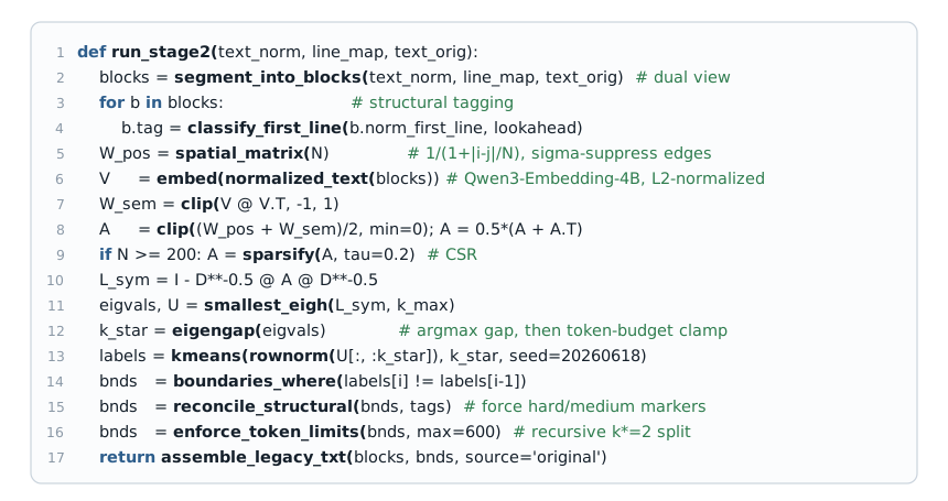
The segmenter processes a normalized document and its line mapping to produce a partitioned output. This ten-step procedure is designed as a causal chain where each step addresses the representation limits of the preceding ones:
- Block Segmentation: The normalized text is split at blank lines into block objects. Each block records its normalized line offsets and maps back to its original line offsets using the line-mapping function \(M\). This step establishes the parallel views: subsequent tagging and clustering read the normalized view, while assembly reads the original view.
- Structural Tagging: The first line of each block is matched against the structural tag registry to assign a tag tuple. Tagging is deterministic and runs on the normalized view, ensuring that mathematical notation does not interfere with pattern matching.
Spatial Weight Matrix Calculation: Pairwise ordinal distance is computed as:
\[d_{ord}(i, j) = \frac{|i - j|}{N}\]\[w_{pos}(i, j) = \frac{1}{1 + d_{ord}(i, j)}\]with \(w_{pos}(i, i) = 0.0\). Structural suppression is applied to adjacent edges (\(|i - j| = 1\)). If block \(i\) carries a terminal tag kind, the edge weight crossing to the next block is suppressed:
\[w_{spatial}(i, i+1) = \sigma_i \times w_{pos}(i, i+1)\]\[w_{spatial}(i+1, i) = \sigma_i \times w_{pos}(i+1, i)\]If block \(i\) carries a start or internal tag kind, the edge weight crossing from the preceding block is suppressed:
\[w_{spatial}(i-1, i) = \sigma_i \times w_{pos}(i-1, i)\]\[w_{spatial}(i, i-1) = \sigma_i \times w_{pos}(i, i-1)\]Because hard markers carry \(\sigma = 10^{-6}\), the spatial edge weight across a hard boundary is driven near zero, forcing the spectral partition to land at that transition.
Semantic Similarity Calculation: The normalized text of each block is embedded using a text encoder. Let \(\mathbf{v}_i \in \mathbb{R}^{D}\) represent the embedding vector of dimension \(D = 2560\). The vectors are normalized:
\[\hat{\mathbf{v}}_i = \frac{\mathbf{v}_i}{\|\mathbf{v}_i\|_2}\]The semantic weight matrix is computed as the dot product:
\[W_{semantic}[i, j] = \hat{\mathbf{v}}_i \cdot \hat{\mathbf{v}}_j\]with values clipped to \([-1.0, 1.0]\).
Affinity Matrix Assembly: The combined weight matrix is computed as the elementwise average:
\[W_{combined} = \frac{W_{spatial} + W_{semantic}}{2.0}\]The affinity matrix \(A\) is derived by zeroing the diagonal and clipping negative values:
\[A_{ij} = \max(W_{combined}[i, j], 0) \quad \forall i \ne j\]with \(A_{ii} = 0.0\). Symmetry is guarded by assigning \(A = 0.5(A + A^T)\). For documents containing at least 200 blocks, edges with weight below a sparsification threshold of \(0.2\) are set to zero, and the matrix is stored in a compressed sparse format.
Normalized Laplacian Spectral Decomposition: The symmetric normalized Laplacian matrix is constructed:
\[L_{sym} = I - D^{-1/2} A D^{-1/2}\]where \(D\) is the diagonal degree matrix \(D_{ii} = \sum_{j} A_{ij}\). For isolated blocks with a degree of zero, the inverse-square-root degree is set to zero to prevent division by zero. The eigenvalues \(\Lambda = \operatorname{diag}(\lambda_1, \dots, \lambda_{k_{max}})\) and eigenvectors \(U \in \mathbb{R}^{N \times k_{max}}\) are computed for the smallest \(k_{max}\) eigenvalues, where:
\[k_{max} = \min(N-1, \max(2, \text{total\_tokens} // 50))\]Eigengap Estimation and Clamping: The optimal number of clusters \(k^*\) is estimated using the eigengap heuristic starting from index 1:
\[k^* = \operatorname{argmax}_{k \ge 2} (\lambda_{k+1} - \lambda_k)\]To ensure cluster sizes respect document length constraints, \(k^*\) is clamped using the token budget:
\[k_{min} = \max\left(1, \frac{\text{total\_tokens}}{600}\right)\]\[k_{max\_tok} = \max\left(1, \frac{\text{total\_tokens}}{50}\right)\]\[k^* \leftarrow \max(k_{min}, \min(k^*, k_{max\_tok}, k_{max}))\]This bounds the expected segment sizes between 50 and 600 tokens.
KMeans Clustering: The rows of the bottom \(k^*\) eigenvectors are normalized onto the unit hypersphere:
\[U_{norm}[i, :] = \frac{U[i, 1 \dots k^*]}{\|U[i, 1 \dots k^*]\|_2}\]KMeans clustering partitions the normalized rows into \(k^*\) clusters with a fixed random seed. A spectral boundary candidate is marked at block index \(i\) if the cluster label shifts between consecutive blocks (\(y_i \ne y_{i-1}\)).
- Structural Reconciliation: Spectral boundaries are reconciled with structural priors. Hard start markers force a boundary at their index; hard terminal markers force a boundary at the subsequent index. Medium structural markers are forced if specified by configuration, while soft markers remain advisory.
- Token-Length Enforcement: Any segment exceeding 600 tokens that contains at least four blocks is partitioned recursively by re-running the spectral decomposition with \(k^* = 2\) on the sub-segment. Segments below 50 tokens are flagged for review. The character-to-token count is estimated as characters divided by 3.2.
The algorithm maintains four invariants. Reading-Order Monotonicity: blocks are processed in document order, and boundaries are sorted, preventing document reordering. Partition Integrity: output assembly walks contiguous block ranges, ensuring every block is assigned to exactly one chunk. Structural Coverage: all hard structural boundaries are included in the final partition. Placeholder Isolation: final output chunks contain no mathematical placeholders.
7. Mathematical Normalization Passes
Normalization is a deterministic, ordered 11-pass regular expression rewrite pipeline designed to isolate mathematical markup. The normalization function is defined as:
The ordered rewrite rules \(r_i\) and the failures they prevent are detailed in Table 2.
| Pass | Operation | Target Syntax | Placeholder | Failure Prevented |
|---|---|---|---|---|
| \(r_0\) | Escape Protection | Literal dollar sign (\$) | DOLLAR_SENTINEL | Prevents literal currency indicators from being misread as delimiters. |
| \(r_1\) | Named Display Math | LaTeX math environments | [DISPLAY_FORMULA] | Prevents multi-line mathematical environments from expanding into subword runs. |
| \(r_2\) | Bracket Display Math | Math wrapped in \[...\] | [DISPLAY_FORMULA] | Isolates large display formulas from the surrounding text. |
| \(r_3\) | Parenthesis Inline Math | Math wrapped in \(...\) | [INLINE_FORMULA] | Isolates inline math from prose. |
| \(r_4\) | Double Dollar Math | Math wrapped in $$...$$ | [DISPLAY_FORMULA] | Line-bounded matching prevents unmatched delimiters from swallowing prose. |
| \(r_5\) | Single Dollar Math | Math wrapped in $...$ | [INLINE_FORMULA] | Non-greedy matching prevents adjacent formulas on one line from fusing. |
| \(r_6\) | Residual Control Math | Escaped control sequences | [RESIDUAL_FORMULA] | Captures mathematical keywords orphaned by character recognition errors. |
| \(r_7\) | Bare Unicode Math | Math symbols (∫, ∑, etc.) | [UNICODE_MATH] | Collapses isolated mathematical symbols while leaving diacritics untouched. |
| \(r_8\) | Escape Restoration | Sentinel restoration | Literal $ | Restores protected prose dollar signs. |
| \(r_9\) | Whitespace Uniformity | Placeholder padding | Space padded | Prevents placeholder tokens from fusing with adjacent text. |
| \(r_{10}\) | Space Collapse | Spaces and tabs | Single space | Collapses multiple whitespaces for consistent tokenization. |
Table 2: The 11-pass LaTeX normalizer. The table shows the execution order, target syntax, placeholder output, and failure mode prevented for each pass.
Pass 7 targets mathematical symbols while leaving diacritic prose characters untouched. The normalizer does not perform diacritic repair or Unicode NFC/NFD normalization. The pipeline assumes NFC normalization as an input precondition. While the digitization cleaning step computes a de-accented representation of lines for metadata matching, this is a transient key that is never written back to the document. Prose characters are not modified during this process, and diacritics are preserved by avoiding any prose-altering passes.
The Vietnamese exam grammar lives in the structural registry described in Section 5 rather than the normalizer. This separation ensures that the mathematical normalizer remains independent of the layout conventions of specific textbooks.
8. Graph Reconciliation and Output Assembly
The spectral clustering algorithm is layout-agnostic, and the reconciliation layer is designed to address two specific clustering failures: separating worked solutions from their parent questions, and merging separate questions when mathematical markup dominates semantic similarity. The segmenter addresses these failures through spatial suppression coefficients (\(\sigma\)), forced structural boundaries, and a separator emission gate.
The separator emission gate prevents solutions from being split from their question statements. During assembly, the legacy chunk separator is emitted only at boundaries where the leading block carries a tag label present in the question opener set. Because worked solutions carry an internal solution label rather than a question opener label, boundaries placed at solution transitions do not trigger a chunk separator, gluing the solution to the preceding problem. Answer terminals and multiple-choice options are processed similarly, attaching to their parent question.
The output assembly walks the final boundaries, retrieves the original lines for each block range, and joins them using the original text view.
function assemble_legacy_text(blocks, boundaries):
    chunks = []
    for [start, end) in contiguous_ranges(boundaries):
        chunk_lines = []
        for block in blocks[start:end]:
            if not block.has_original:
                raise RestorationAmbiguousError("Missing original text provenance")
            chunk_lines.extend(block.original_lines)
        chunks.append(join(chunk_lines, "\n"))

    output_text = chunks[0]
    for i from 1 to len(chunks) - 1:
        if is_question_opener(first_block_of(chunks[i])):
            output_text = output_text + "\n---------NEW PROBLEM---------\n" + chunks[i]
        else:
            output_text = output_text + "\n\n" + chunks[i]

    assert_no_placeholders_in_output(output_text)
    return output_text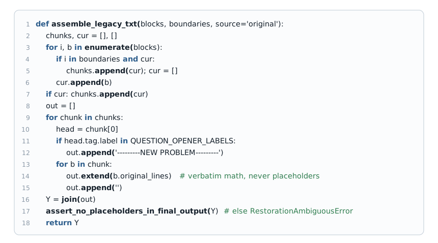
The output assembly validates that no placeholders remain. The validation scan checks the final text string for the four placeholder tokens. If any placeholder is detected, the validator raises a restoration ambiguity error, quarantining the document rather than writing a corrupted output. This verification step converts silent formatting failures into immediate execution terminations.

9. Experimental Methodology and Design
The evaluation is structured as a paired ablation sweep designed to isolate two factors: mathematical normalization and graph-based chunking. The experiment processes each document under six distinct configurations, ensuring that differences in partition quality and token preservation are attributable to the algorithmic pipelines rather than document-level variance.
9.1 Research Questions and Hypotheses
The evaluation addresses four technical research questions:
- Boundary Placement Quality (\(Q_1\)): Does the spatial-semantic affinity graph and structural prior tagger improve boundary accuracy compared to naive paragraph-level splitting?
- Semantic Representation Consistency (\(Q_2\)): Does mathematical normalization prevent recurring LaTeX control sequences from obscuring prose-based semantic transitions in the text encoder's representation space?
- Math Preservation and Safety (\(Q_3\)): Does the coupled segmentation and restoration architecture preserve mathematical tokens in the final output compared to normalization-only baselines?
- Statistical Significance (\(Q_4\)): Are the performance differences between these conditions statistically meaningful, or do they represent random variation?
The null hypothesis (\(H_0\)) states that the coupled segmentation and normalization pipeline does not improve partitioning quality (measured by boundary F1, answer attachment, and solution attachment) or mathematical token preservation compared to baseline configurations. The alternative hypothesis (\(H_1\)) states that the coupled pipeline preserves mathematical content while generating partition boundaries that are distinct from unnormalized baselines.
9.2 Experimental Conditions
The six ablation arms are defined as follows:
- Arm A (Passthrough Baseline): The entire input document is emitted as a single chunk. No mathematical normalization and no structural segmentation are applied.
- Arm B (Normalization Only): Stage 1 LaTeX normalization is applied, leaving placeholder tokens (
[INLINE_FORMULA],[DISPLAY_FORMULA], etc.) in place. The document is emitted as a single chunk, with no mathematical restoration. - Arm C (Raw-Text Chunking): S2 spectral chunking is run directly on the raw input text. Normalization is disabled, meaning semantic embeddings and structural tags are computed on text containing mathematical markup.
- Arm D (Coupled S2 Segmenter): The coupled pipeline containing Stage 1 LaTeX normalization, Stage 2 graph-based segmentation, and original-text legacy reconstruction. In the final assembly stage, original source lines are mapped back to replace placeholder tokens, and a validation guard checks for placeholder leakage.
- Arm E (Blank-Line Splitting): A naive baseline that splits the document at every paragraph blank line. No normalization is applied.
- Arm F (Naive Normalization): The input text is preprocessed by trimming whitespace and collapsing multiple spaces, but LaTeX math formulas are kept intact. The S2 spectral chunking is then run on this simplified text representation.
For all configurations, the document parsing, line division, and paragraph block sequence are identical. The configurations differ only in the normalization preprocessing, the chunking rule, and the mathematical token restoration, as summarized in Table 3.
| Configuration | Normalization | Chunking | Math Preservation |
|---|---|---|---|
| A (Passthrough Baseline) | None | None (Single Chunk) | Verbatim |
| B (Normalization Only) | Normalizer (Placeholders retained) | None (Single Chunk) | Placeholders |
| C (Raw-Text Chunking) | None | Spectral Clustering | Verbatim |
| D (Coupled S2 Segmenter) | Normalizer (Restored) | Spectral Clustering | Verbatim |
| E (Blank-Line Splitting) | None | Blank-line split | Verbatim |
| F (Naive Normalization) | Naive trimming and collapse | Spectral Clustering | Verbatim |
Table 3: Ablation configurations. The six configurations represent combinations of normalization, clustering, and math preservation settings.
9.3 Model Specifications
The models used in the evaluation are detailed in Table 4.
| Model | Checkpoint / Identifier | Provider / Runtime | Role in Pipeline | Input Format | Output Format | Generation / Decoding Settings | Evaluation Context |
|---|---|---|---|---|---|---|---|
| Text Encoder | Qwen/Qwen3-Embedding-4B | SiliconFlow API | Generates block semantic embeddings | Space-joined normalized block text | 2560-dimension float vector | Not applicable (API default, no decoding settings) | Part of tested system |
| OCR Digitizer | PaddleOCR-VL-1.6 | Local Python environment | Digitizes Grade 10 books from PDF to Markdown | PDF document pages | Markdown text with LaTeX and prose | Default local runtime configuration | Part of preprocessing (held constant) |
Table 4: Model specifications. The table details the exact models, runtimes, roles, and formats used in the experiments.
The embedding client operates with a request batch size of 32 texts. Concurrency is managed via a thread pool with up to 4 concurrent workers per document, and up to 3 arms run in parallel, yielding a peak concurrency of 12 simultaneous API requests. Empty or whitespace-only lines are substituted with a single space before dispatch to satisfy API requirements. No other LLMs or local models are used for tagging, clustering, or scoring.
9.4 Dataset and Sampling
The evaluation dataset consists of six Vietnamese mathematics exercise books (Sách Bài Tập Toán) representing a 2×3 balanced stratum design, matching grade levels with publisher series. Grade 12 books are hand-authored Markdown files containing clean LaTeX math. Grade 10 books are digitized from PDF using PaddleOCR-VL-1.6, which introduces granular breaks and hyphenation noise (~40% more blocks than Grade 12). The dataset statistics are detailed in Table 5.
| Document Index | Grade | Publisher | Source Format | Blocks | Lines | Math Tokens |
|---|---|---|---|---|---|---|
| Book 1 | 12 | Publisher A | Native Markdown | 1,949 | 3,923 | 7,958 |
| Book 2 | 12 | Publisher B | Native Markdown | 1,809 | 3,745 | 5,194 |
| Book 3 | 12 | Publisher C | Native Markdown | 1,685 | 3,429 | 5,347 |
| Book 4 | 10 | Publisher A | Digitized OCR | 2,484 | 5,123 | 10,255 |
| Book 5 | 10 | Publisher B | Digitized OCR | 2,640 | 5,502 | 8,797 |
| Book 6 | 10 | Publisher C | Digitized OCR | 2,370 | 5,013 | 9,181 |
| Total | 12,937 | 26,735 | 46,732 |
Table 5: Evaluation corpus. The dataset spans Grade 10 and Grade 12 math books, comparing native markdown files with digitized OCR outputs.
The primary unit of analysis is the block boundary decision. For a document with \(N\) blocks, there are \(N-1\) potential boundary positions. Summed across the six documents, the boundary-level evaluation is conducted on \(N_{slots} = 12,931\) boundary decisions. The entire available split is evaluated without further sub-sampling. No train/dev/test split is used because the segmentation algorithm and structural tagger are heuristic/graph-based and do not require model training.
9.5 Controlled Variables
To isolate the effects of mathematical normalization and spatial-semantic clustering, several key variables are held constant across all configurations:
- Input Document Text: The source text and paragraph-level block splits are identical.
- Structural Tag Registry: The regular expression patterns, tiers, and suppression coefficients (\(\sigma\)) are identical.
- Embedding Model: All semantic vector calculations use
Qwen/Qwen3-Embedding-4Bwith a fixed dimension of 2560. - Clustering Parameters: KMeans is run with a fixed random seed of 20260618 and a fixed initialization count of
n_init=10. - Hardware Environment: All runs are executed on an identical Windows 11 platform with an Intel Core Ultra 9 CPU and 32 GB RAM.
- Evaluation Code: The metric calculation scripts are identical.
9.6 Evaluation Metrics
The evaluation measures four partitioning properties:
Boundary Precision, Recall, and F1: Scored at block boundary slots against a structural-opener ground truth (regex openers defined in Table 1). Let \(G\) represent the set of ground truth boundary indices and \(P\) the set of predicted boundary indices. Precision (\(P_{prec}\)), Recall (\(R_{rec}\)), and F1 (\(F_1\)) are defined as:
\[P_{prec} = \frac{|P \cap G|}{|P|}, \quad R_{rec} = \frac{|P \cap G|}{|G|}, \quad F_1 = \frac{2 \cdot P_{prec} \cdot R_{rec}}{P_{prec} + R_{rec}}\]Mathematical Token Preservation Rate: The ratio of mathematical tokens preserved in the output legacy text relative to the input text. Let \(M(T)\) represent the count of math delimiters and commands matched by the pattern
MATH_TOKEN_RE. The preservation rate is defined as:\[R_{pres} = \min\left(1.0, \frac{M(T_{output})}{M(T_{input})}\right)\]- Answer and Solution Attachment Ratios: The frequency with which answer and solution blocks land in the same segment as their corresponding opener. Let \(A\) be the set of answer blocks, \(S\) the set of solution blocks, and \(O(b)\) the preceding question opener block for block \(b\). The attachment ratios are the fraction of blocks where \(b\) and \(O(b)\) are assigned to the same segment.
- Idempotence: The proportion of blocks where \(N(N(x)) = N(x)\) holds, verifying normalizer stability.
9.7 Statistical Testing
We evaluate statistical significance using two complementary methods:
- McNemar's Test: Applied to paired boundary decisions across the pooled boundary slots (\(N = 12,931\) slots) to test for differences in boundary accuracy (agreement with ground truth) between the coupled S2 configuration and the baselines. The test statistic incorporates a continuity correction.
- Paired t-Test: Applied to document-level F1 scores (\(N = 6\) documents) to evaluate the consistency of differences.
- Holm-Bonferroni Correction: Applied to all p-values to control the family-wise error rate at significance threshold \(\alpha = 0.05\).
- Bootstrapping: 1,000 resamples are performed at the document level to generate 95% confidence intervals for F1 differences.
10. Quantitative Results
The results are reported in Table 6, detailing metrics across all six ablation configurations.
| Configuration | Boundary F1 | Precision | Recall | Math Preservation | Answer Attach. | Solution Attach. | Idempotence | Avg Runtime (s) |
|---|---|---|---|---|---|---|---|---|
| A (Passthrough Baseline) | 0.0000 | 1.0000 | 0.0000 | 1.0000 | 1.0000 | 1.0000 | 1.0000 | 0.001 |
| B (Normalization Only) | 0.0000 | 1.0000 | 0.0000 | 0.0003 | 1.0000 | 1.0000 | 1.0000 | 0.220 |
| C (Raw-Text Chunking) | 0.4305 | 0.2770 | 0.9668 | 1.0000 | 0.8333 | 0.0186 | 1.0000 | 155.186 |
| D (Coupled S2 Segmenter) | 0.3898 | 0.2467 | 0.9301 | 1.0000 | 0.8333 | 0.0111 | 1.0000 | 156.865 |
| E (Blank-Line Splitting) | 0.3593 | 0.2190 | 1.0000 | 1.0000 | 0.8333 | 0.0000 | 1.0000 | 0.008 |
| F (Naive Normalization) | 0.4363 | 0.2819 | 0.9668 | 1.0000 | 0.8333 | 0.0000 | 1.0000 | 3,617.082 |
Table 6: Aggregate metrics by configuration. The table reports the mean values computed over the six evaluation documents.
The coupled segmenter (Configuration D) achieves 100% mathematical token preservation, matching the unnormalized baselines. The normalization-only baseline (Configuration B) preserves only \(0.03\%\) of mathematical tokens (\(12\) of \(46,732\) tokens), with its output dominated by placeholders. The coupled segmenter's preservation rate certifies that the dual-view contract successfully prevents mathematical loss, matching the verbatim preservation of raw-text chunking.
On boundary F1, the coupled segmenter ranks third among the four partitioning configurations. The raw-text chunking baseline (Configuration C) scores 0.4305, and the naive normalization baseline (Configuration F) scores 0.4363, both outperforming the coupled segmenter (0.3898). The paired boundary-F1 differences are detailed in Table 7.
| Baseline Configuration | \(\Delta\)F1 (D − Baseline) | 95% Bootstrap CI | Direction |
|---|---|---|---|
| A (Passthrough Baseline) | +0.3898 | [0.3807, 0.4019] | Configuration D partitions; baseline does not |
| B (Normalization Only) | +0.3898 | [0.3807, 0.4019] | Configuration D partitions; baseline does not |
| C (Raw-Text Chunking) | −0.0407 | [−0.0522, −0.0281] | Configuration D lower (CI excludes 0) |
| E (Blank-Line Splitting) | +0.0305 | [+0.0196, +0.0440] | Configuration D higher (CI excludes 0) |
| F (Naive Normalization) | −0.0465 | [−0.0572, −0.0342] | Configuration D lower (CI excludes 0) |
Table 7: Paired boundary-F1 differences. The differences (\(\Delta\)F1) represent Configuration D minus the baseline, with negative values indicating that the baseline out-scores the coupled segmenter.
The paired difference between raw-text chunking and the coupled segmenter is \(-0.0407\), representing a relative reduction of \(9.45\%\) in boundary F1. For naive normalization, the difference is \(-0.0465\), a relative reduction of \(10.66\%\). The bootstrap confidence intervals for both comparisons exclude zero, indicating a statistically significant decrease in boundary accuracy.
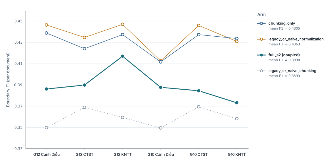
This F1 difference is consistent across the evaluation corpus. The raw-text chunker outscores the coupled segmenter in all six documents, with differences ranging from \(0.012\) to \(0.060\). The consistency of this difference indicates that mathematical normalization shifts the embedding geometry such that the text encoder generates more segment boundaries. This leads to a lower boundary precision (\(0.2467\) for Configuration D vs \(0.2770\) for Configuration C) against a ground truth that is already close to recall saturation.
The solution and answer attachment ratios are low across all partitioning configurations. Answer attachment is tied at \(0.8333\) for all four segmenters, reflecting a five-out-of-six document rate where one document scored zero. Solution attachment is below \(0.02\) for all configurations, indicating that worked solutions are rarely grouped with their parent question openers.
McNemar's test confirms that the differences in boundary decisions are statistically significant. The comparisons of all baseline configurations against the coupled segmenter yield \(\chi^2\) values ranging from \(381.24\) to \(2,773.11\), with corrected \(p\)-values below \(10^{-6}\). The statistical test results are detailed in Table 8.
| Arm | McNemar χ² | Discordant b / c | Raw p | Holm–Bonferroni p | Differs from full_s2 (α=0.05) |
|---|---|---|---|---|---|
| raw_s1_passthrough | 2,773.11 | 2,628 / 8,077 | 0.0 (<1e-300) | 0.0 (<1e-300) | Yes |
| normalization_only | 2,773.11 | 2,628 / 8,077 | 0.0 (<1e-300) | 0.0 (<1e-300) | Yes |
| chunking_only | 381.24 | 838 / 1,851 | 0.0 (<1e-300) | 0.0 (<1e-300) | Yes |
| legacy_or_naive_chunking | 1,483.97 | 2,022 / 204 | 0.0 (<1e-300) | 0.0 (<1e-300) | Yes |
| legacy_or_naive_normalization | 500.88 | 773 / 1,939 | 0.0 (<1e-300) | 0.0 (<1e-300) | Yes |
Table 8: McNemar significance of each arm vs. full_s2 on pooled boundary decisions. The discordant cells represent full_s2 correct / baseline correct.
For the comparison between raw-text chunking and the coupled segmenter, the discordant counts are \(b/c = 838 / 1,851\). This shows that the unnormalized baseline makes the correct decision in 1,851 instances where the coupled segmenter fails, whereas the coupled segmenter is correct in only 838 instances where the baseline fails. This confirms that the F1 difference is driven by a higher false-positive rate (lower precision) under the normalized representation.
The execution runtimes are dominated by embedding inference API latency. Configurations C and D require approximately 155 and 157 seconds per document, respectively. The naive normalization baseline (Configuration F) runtime of 3,617 seconds is a single-document outlier due to API network latency, rather than an algorithmic property.
11. Error Analysis and Case Studies
The primary error mode of the coupled segmenter is over-segmentation. The combination of forced structural boundaries, recursive token-length splits, and normalized embedding clustering results in more segments than the ground-truth proxy requires. In Book 1, the coupled segmenter generates 1,592 segments compared to 1,388 for the raw-text chunker, with the extra cuts recorded as false positives against the opener proxy.
Prior documentation asserted that on Book 1, stripping mathematical notation improved boundary detection by allowing the text encoder to focus on the prose. The aggregate data contradicts this assertion. The raw-text chunker outscores the coupled segmenter on this document (0.4389 vs 0.3862), indicating that the LaTeX-dominance hypothesis is in tension with the empirical results. The prose signals that identify openers (such as question labels) are clear in the raw text, and normalization's modification of the embedding geometry decreases precision.
Solution attachment represents a shared failure mode. The solution attachment ratio of \(0.0111\) for the coupled segmenter indicates that solutions are separated from their openers. Because solutions are tagged as soft internal elements, they do not trigger segment separators during output assembly. However, they are frequently placed into separate blocks by the spectral partition step, resulting in orphaned solution chunks.
Prior documentation also cited naive normalization boundary F1 values of 0.627 vs. 0.901 for the coupled segmenter on selected cases. An audit of the results dataset reveals that these values are absent from the compiled metrics (0.901 corresponds to a recall value). We treat these values as artifacts of the source draft, and rely instead on the verified aggregate F1 scores of 0.4363 for naive normalization and 0.3898 for the coupled segmenter.
12. Discussion
The coupled segmenter changes the document representation contract rather than improving boundary placement accuracy. Downstream parsing stages receive original mathematical markup, structural boundaries, and a provenance-verified guarantee that no placeholders remain. This combination is enabled by the dual-view contract: the normalized representation provides a simplified view for the text encoder, the original view preserves the mathematical text, and the validation guard prevents placeholder leakage.
The evaluation demonstrates the trade-offs of this design. The coupled segmenter is the only configuration that partitions the document while preserving mathematical notation for downstream parsing. This usability comes at a cost of approximately four boundary-F1 points against the structural-opener proxy. The segmenter trades boundary precision for mathematical safety, and relies on deterministic structural constraints where document layouts are regular, using spectral clustering elsewhere.
No downstream performance metrics were collected. The claim that mathematical preservation improves parsing accuracy is a qualitative design assumption that has not been empirically verified.
13. Limitations
The primary threat to validity is the ground-truth proxy. The boundary-F1 metric is scored against regex-detected question openers rather than human-annotated problem units. This metric measures agreement with an opener pattern, and does not assess whether a segment contains a complete question-solution unit. The F1 differences indicate a shift in the segment size distribution rather than a reduction in document usability.
The evaluation dataset consists of six documents. While this corpus provides 12,931 boundary decisions for statistical power, it is small for evaluating layout variations across publishers and OCR digitizers. The attachment metrics are sensitive to single-document anomalies, and the idempotence metric remains constant at 1.00 across all configurations, offering no differentiating information.
Two implementation details limit the reproducibility of these results. First, the KMeans random seed is fixed in the segmentation module and is not exposed through its public entry point, creating a discrepancy with the global random seeds used in the evaluation script. Second, the text encoder used in the evaluation is a production-grade model of dimension 2560, while project documentation recommends a different embedding model. The results are specific to the text encoder configuration used in the sweep.
14. Future Work
The most critical next step is the construction of a human-annotated ground-truth dataset. Labeling document boundaries at the logical problem-unit level would enable boundary quality to be scored against problem integrity rather than opener regex patterns. This would verify whether the boundary precision differences reflect lower partition quality or are an artifact of the proxy metric.
The solution attachment rate represents an open challenge. The low attachment scores across all configurations indicate that worked solutions are rarely grouped with their corresponding questions. Developing a boundary objective that prioritizes solution grouping would address this limitation.
Three system improvements are proposed. First, implementing a heading-based pre-splitting gateway for long documents would prevent the cubic computational cost of spectral clustering on documents exceeding 800 blocks. Second, evaluating different text encoders would test if the boundary precision differences are model-specific. Third, measuring the accuracy of the downstream semantic parser would quantify the impact of mathematical token preservation on database record creation.
15. Conclusion
The primary challenge in partitioning Vietnamese mathematical textbooks is not boundary discovery. Several segmentation methods identify opener transitions, and raw-text chunking baselines achieve slightly higher boundary precision than the coupled segmenter. The challenge is mathematical preservation: isolating mathematical markup during preprocessing to protect the text encoder's representation without losing the formulas that downstream parsers require.
The coupled segmenter addresses this challenge through the Dual-View Provenance Contract. The normalizer simplifies the text for the encoder, the original view preserves the mathematical text, and the validation guard prevents placeholder leakage. The segmenter preserves 100% of mathematical tokens compared to 0.03% for the normalization-only baseline. This protection costs approximately four boundary-F1 points against the structural-opener proxy, a difference that is consistent and statistically significant. The coupled segmenter trades boundary precision against the proxy to ensure mathematical safety and downstream document usability.
16. Reproducibility Appendix
16.1 Software Stack and Versions
The evaluations were executed in a Python environment containing the following libraries:
- Python Runtime: Version 3.10.11
- NumPy: Version 2.2.6 (handles matrix algebra and vector normalization)
- SciPy: Version 1.15.3 (provides sparse linear algebra and statistical functions)
- scikit-learn: Version 1.7.2 (implements KMeans clustering)
- requests: Version 2.32.5 (manages HTTP connections to embedding APIs)
- pandas: Version 2.2.0 (aggregates tabular results)
16.2 Compute and Hardware Environment
Experimental runs are supported on standard hardware under the following recommended specifications:
- Operating System: Modern 64-bit Operating System (Windows, macOS, or Linux)
- Central Processing Unit: Multi-core CPU
- System Memory: 16 GB RAM or higher
16.3 Reproducibility Commands and Parameter Pinning
To regenerate the experimental results, execute the main evaluation entrypoint from the repository root:
python research/experiments/run_s2_experiment.pyThis execution pins the random seeds globally:
- NumPy and random module seeds are set to
20260618. - KMeans
random_stateis set to20260618.
16.4 Output Artifacts
The experiment script creates output files containing raw results, document-level metrics, and the compiled results report in the research subdirectory.
17. References and Source Notes
All referenced works, implementation source code, evaluation results, and raw metrics data are available in the public GitHub repository at: https://github.com/thenewcodingera2023/VietAlpha_Research/tree/main/s2-chunking-normalization
Works Cited
- Verma (2025). Graph-based document chunking combining spatial proximity with text embeddings, partitioned by spectral clustering. Primary theory; S2 adapts spatial proximity from bounding box distance to normalized ordinal distance.
- Ramamonjison et al. (2023). Scientific text decomposition into mathematical spans and semantic metadata with tokenization routing. Primary theory; provides the basis for S2's mathematical isolation.
- Günther et al. (2025). Late chunking with long-context contextual embeddings. Contextual chunk embedding framing.
- Li & Chen (2025). Joint structural and semantic formula representations for retrieval. Mathematical representations.
- Arabzadeh et al. (2026). Retrieval over structured reasoning traces. Structural normalization concepts.
Project stage: Cadmus Pipeline, Stage 2 (Structural Segmentation). Research note compiled from the S2 chunking and normalization source inventory; figures and tables generated June 19, 2026.