Research Note

Neural networks and Vietnamese maths

May 23, 2026 · Harry Tran

This paper explores how multivariable calculus works in neural network training. Each concept is derived and explored. The closing sections then turn to a problem the training analysis sets aside, the faithful representation of the input itself, taken up for the case of mathematics written in natural language.

Neural Network Architecture

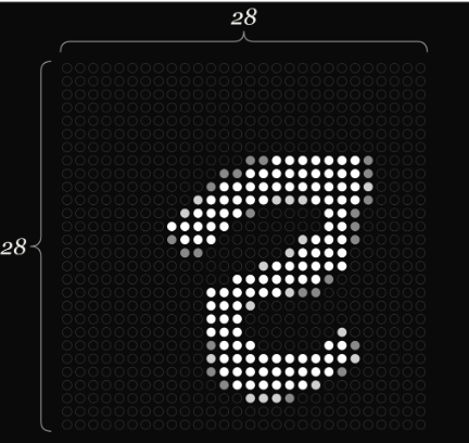
Neural networks consist of neurons and layers. Neurons are data points that hold numbers that represent a piece of information in the network. The number within a neuron is called an "activation". Together, these "activations" make up the unique properties of each neuron. A group of neurons makes up a layer. Consider a neural network that specializes in identifying handwritten text, and is presented with a 28x28 image of a single written number "2".

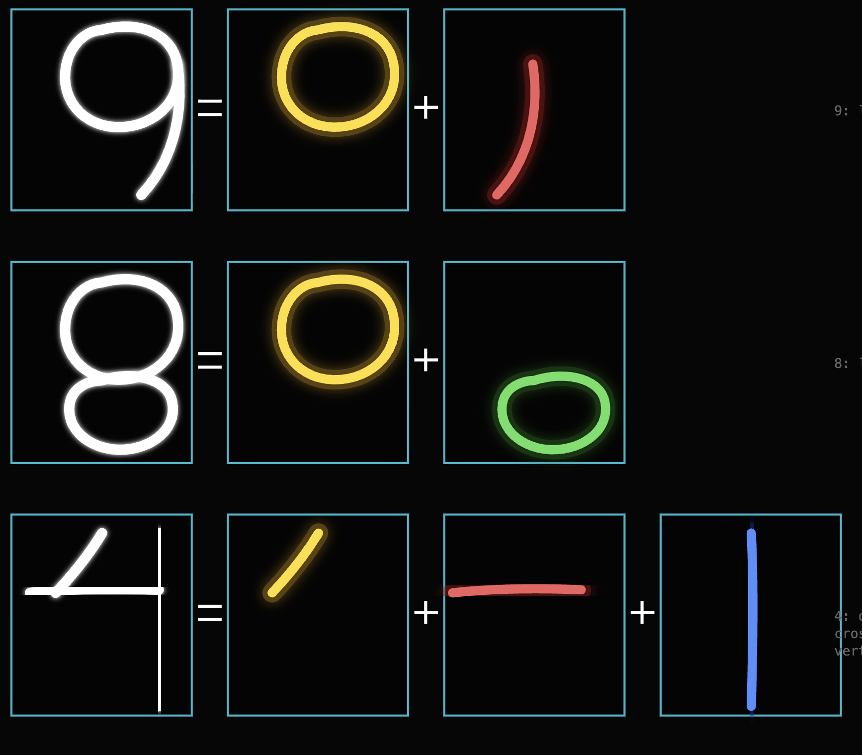
The image will be processed as an input layer pixel by pixel, and each of the 784 neurons holds unique activation values that activate specific patterns of neurons in the next activation layer. Machine learning models recognize patterns from the ground up through separate components that compose the input. For instance, the number seven consists of a "—" and "/," and 1 also consists of "—" and "I," while four holds up to three distinct strokes.

These patterns correspond with a neuron within the layers of neural networks. So when data is fed into an AI, neurons that share the closest resemblance activate, and every layer repeats this cycle until the end, where the neurons narrow down to a specific subset of output that is most accurate. Therefore, a network with more layers may yield higher accuracy because they have more turns to eliminate incorrect patterns before arriving at the final output layer.

Forward Pass

Each neuron in the next layer not only receives a signal but also computes a score. That score is a weighted sum of every input neuron's activation value. Pixels that help detect a stroke have higher weights. Irrelevant pixels score lower or even zero. A constant (bias) is added to shift the score up or down. This weighted sum, along with bias, is an affine transformation. Everything the neural network "understands" is stored in weights. So in AI training, weights are adjusted to move the model's output towards a desired outcome. The following equation demonstrates the concept:

\(z\) is the pre-activation while \(a = \sigma(z)\) becomes post-activation. Every input pixel value \(a\) gets multiplied by the weight \(w\) and added to \(b\). The nonlinear activation of \(\sigma\) is applied (Nair & Hinton, 2010):

ReLU is not differentiable at \(z = 0\). Throughout this paper we adopt the implementation convention

so that \(\sigma'(0)\) is treated as a chosen subgradient value. This matches the behavior of common deep learning frameworks and lets us write \(\sigma'(z)\) in subsequent gradient expressions without piecewise qualifications.

Network Composition and the Loss Function

So the network repeats this mathematical process across every layer. If every layer \(\ell\) performs:

Then the full network is:

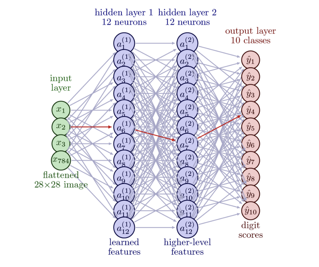
where \(K\) is the total number of affine layers in the network. We reserve \(L\) for the loss function defined below. Hence, 784 neurons from the example model in the input layer will be clamped down to 10 neurons at the output layer (Figure 3):

This dimension translation also accounts for the loss function of the neural network. It measures how wrong the network's output is compared to the correct answer, helping model improvement during training. It's a scalar function of all the trainable parameters:

where \(P\) is the total number of trainable parameters (weights and biases) across all layers. Thus, a simple loss is mean squared error:

where \(\hat{y}\) is the network's predicted score, and \(y\) is the correct label. The goal in training is to make \(L\) as small as possible by adjusting the weights (\(w\)) and biases (\(b\)). The gradient is then used to define the direction of adjustment. The partial derivative \(\partial L / \partial \theta_i\) shows the rate of change of loss with respect to a single parameter \(\theta_i\), holding the rest fixed.

The vector \(\theta \in \R^{P}\) collects every weight \(W^{\ell}_{jk}\) and every bias \(b^{\ell}_j\) across all \(K\) layers, so the gradient has a component for each.

Inside a Single-Neuron Network

The gradient reveals which direction to move each parameter, but it doesn't say how to compute each \(\partial L / \partial \theta_i\). Modern networks contain trillions of weights, meaning that checking each weight and re-running forward passes is computationally impossible. The chain rule becomes useful since \(L\) is a composition of layers; it decomposes every partial derivative into a product of local factors. Consider a network where every layer has one neuron (Figure 4).

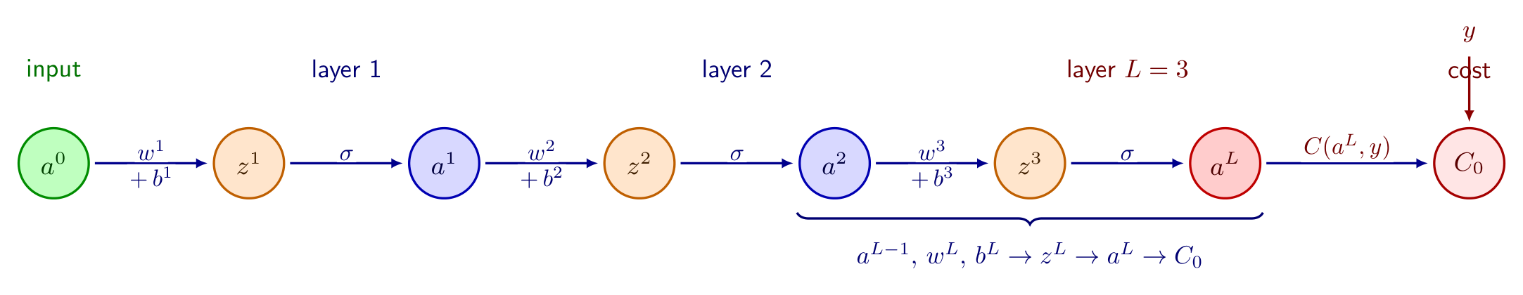
Three affine layers means three weights \(w^{1}, w^{2}, w^{3}\), three biases \(b^{1}, b^{2}, b^{3}\), and a chain of scalar activations where \(a^{0}\) is the input. For one training example, the cost is:

where \(K = 3\) and \(y\) is the target. This is the squared-error cost for a single example. The full training loss \(L\) is the average of \(C_0\) over many examples. The final activation is:

where \(\sigma\) is the activation function, \(a^{K}\) is post-activation, and \(z^{K}\) is the affine transformation. The dependency graph for the last two layers in the network is:

We want to know how the change in \(w^{K}\) propagates through to \(C_0\). Chain rule decomposes this into a product of three local derivatives, one for each arrow in the dependency graph:

From \(z^{K} = w^{K} a^{K-1} + b^{K}\), we treat \(a^{K-1}\) and \(b^{K}\) as constants when differentiating with respect to \(w^{K}\):

The second factor:

The third factor:

Combine all of the factors above:

The amount that \(z^{K}\) moves when \(w^{K}\) moves is set by the activation of the upstream neuron. If \(a^{K-1} = 0\) then no change in the weight has any effect on \(z^{K}\). If the upstream neuron fires strongly, then small changes to the weight produce large changes downstream.

Layer Jacobians

However, the scenario above only describes the cost changes with respect to a single weight in a final layer. Sophisticated networks map vector to vector in different dimensions, and the derivative becomes a Jacobian matrix. So the layer \(\ell\) is the matrix \(J^{\ell} \in \R^{n_{\ell} \times n_{\ell-1}}\) with entries:

Row \(i\) and column \(j\) records how much output neuron \(i\) responds to a small change in input neuron \(j\). The full matrix collects all responses at once. Affine transformation and activation also follow a similar manner when expanded to a network of neurons. Recall the operation:

To find how \(z^{\ell}\) responds to a change in \(a^{\ell-1}\), differentiate each output \(z^{\ell}_i = \sum_j W^{\ell}_{ij} a^{\ell-1}_j + b^{\ell}_i\) with respect to each input \(a^{\ell-1}_j\):

Recall the activation function:

Each output \(a^{\ell}_i\) depends only on \(z^{\ell}_i\), not on any other \(z^{\ell}_j\). Therefore:

\(\sigma\) is applied elementwise, thus, the output \(i\) is a function of input \(i\) only in (17). It bears no dependence on \(z^{\ell}_j\) when \(i \neq j\). So \(\partial a^{\ell}_i / \partial z^{\ell}_j = 0\) whenever \(i \neq j\) because the variable isn't present in the expression. The partial derivative of a function with respect to a variable it doesn't contain is zero. So diagonal entries of \(i = j\) are each equal to \(\sigma'(z^{\ell}_i)\) and the Jacobian is diagonal:

Since \(f^{\ell}\) ((5)) is the composition of the activation with the affine transformation, the chain rule gives the full layer Jacobian as the product of the two. Define \(D^{\ell} = \diag\!\left(\sigma'(z^{\ell})\right)\). Then:

The Jacobian of the full network is the chain-rule product of the per-layer Jacobians, written in reverse order so that the leftmost factor corresponds to the final layer acting last on a column vector:

The nonlinear nature of the network lies in the concept that each diagonal factor \(D^{\ell}\) depends on the input \(x\) through the forward pass values \(z^{\ell}\). The Jacobian changes with every input, even though each factor is a fixed matrix at any given input. The activation function maintains the network's expressive capacity and prevents \(J_f\) from reducing to a single matrix.

Backpropagation

Now that the layers have been mapped, the loss \(C_0\) ((11)) needs to respond to multiple weights in each neuron through different layers.

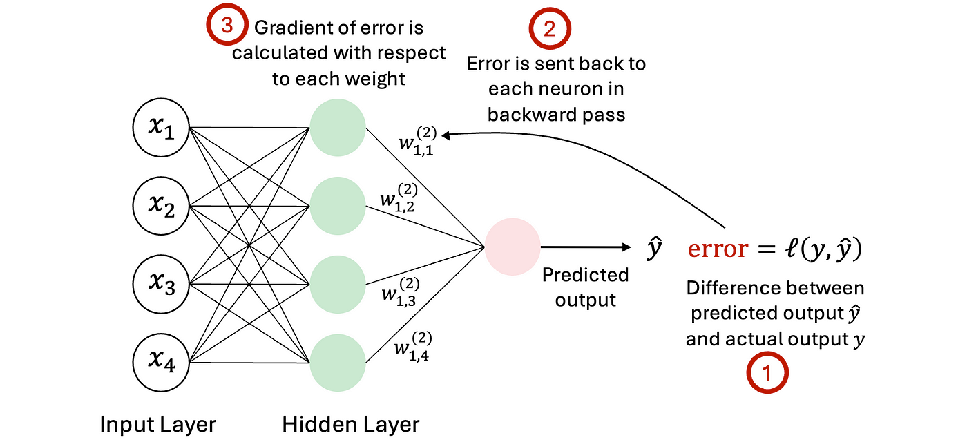
Previously, in a single-neuron network, the activation \(a^{K-1}\) fed into exactly one neuron. There was one path from \(a^{K-1}\) to \(C_0\) (Figure 4), so the chain rule was a single product. In real layers with \(n_K\) output neurons, the activation \(a^{K-1}_k\) of neuron \(k\) goes into every pre-activation \(z^{K}_j\) for every \(j\). Therefore:

So \(a^{K-1}_k\) influences \(C_0\) through \(n_K\) separate paths simultaneously, one through each neuron \(j\). This requires summing the contribution from each path:

Each term in the sum is equivalent to one path through a downstream neuron \(j\). The factor \(\partial C_0 / \partial a^{K}_j\) measures how sensitive the loss is to output neuron \(j\). This is useful for measuring the impact of adjusting specific weights and tracking loss during training. The factor \(\partial a^{K}_j / \partial a^{K-1}_k\) measures how much neuron \(k\) in layer \(K - 1\) moves neuron \(j\) in layer \(K\). We can decompose the second factor:

Substitution back into (21) gives:

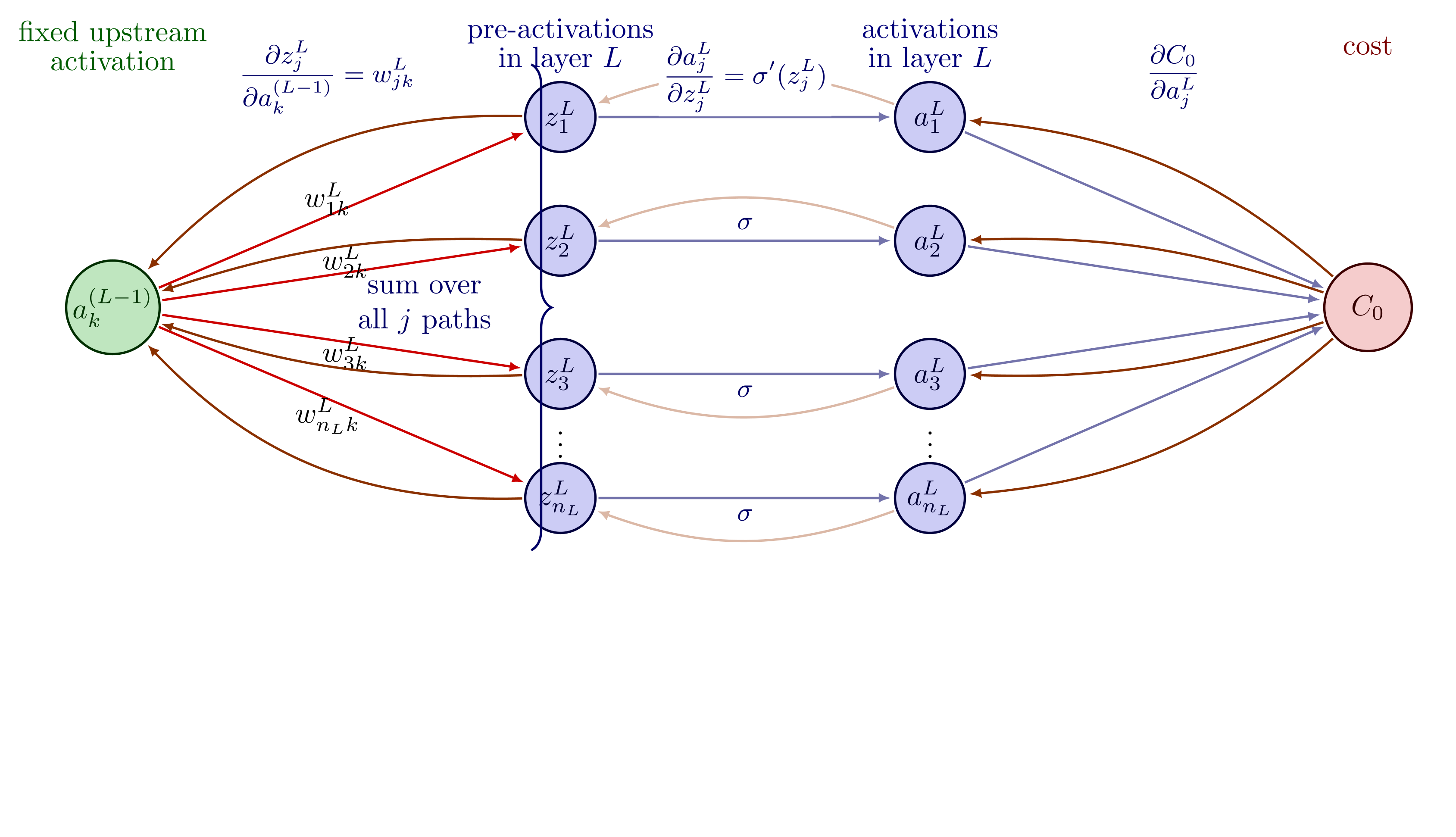
This process altogether is called recursion (Figure 6). The gradient with respect to layer \(K - 1\)'s activation is expressed in computable quantities like weights \(w^{K}_{jk}\) and the forward-pass values \(z^{K}_j\). Each step of the backward pass uses the gradient from the layer above and produces the gradient for the layer below. The sum over \(j\) with \(k\) fixed is going down column \(k\) of the weight matrix \(W^{K}\). Column \(k\) contains all weights that connect upstream neuron \(k\) to every downstream neuron \(j\). In matrix notation, this summation is a multiplication by \((W^{K})\T\). The full backward recursion is:

where \(\delta^{\ell} = \partial C_0 / \partial z^{\ell}\) is the error signal at layer \(\ell\) and \(\odot\) is elementwise multiplication (Rumelhart et al., 1986). \(W^{\ell+1}\) is the weight matrix of the layer above \(\ell\), using their values to route the error backwards in the network. So the recursion demonstrates how sensitive \(C_0\) is to the pre-activations at layer \(\ell\).

However, those are all intermediate quantities in a forward pass and cannot be adjusted. We want to transform the recursion gradient so it is with respect to the weights. Recall that weight \(W^{\ell}_{jk}\) affects \(C_0\) through the path ((20)):

Therefore:

For the second factor, recall \(z^{\ell}_j = \sum_{k} w^{\ell}_{jk}\, a^{\ell-1}_k + b^{\ell}_j\). Differentiating with respect to \(W^{\ell}_{jk}\):

Thus:

Stacking the entries by row \(j\) and column \(k\) gives the matrix form:

The bias gradient follows the same path. Since \(z^{\ell}_j = \sum_{k} w^{\ell}_{jk}\, a^{\ell-1}_k + b^{\ell}_j\), differentiation with respect to \(b^{\ell}_j\) gives \(\partial z^{\ell}_j / \partial b^{\ell}_j = 1\). Therefore:

The recursion in (23) runs from \(\ell = K - 1\) down to \(\ell = 1\), so it requires an initial value \(\delta^{K}\) at the output layer. From the squared-error cost \(C_0 = (a^{K} - y)^2\) in (11), generalized componentwise to a vector output, the output-layer error signal is:

For a minibatch of \(M\) examples, both (24) and (25) are averaged over the \(M\) per-example gradients to give the parameter update direction.

Optimization

The previously introduced loss function \(L(\theta) : \R^{P} \to \R\) ((8)) defines a hypersurface in \(P + 1\) dimensions and its properties.

During normal training rounds \(\nabla L(\theta) \neq 0\) so the gradient moves \(\theta \leftarrow \theta - \eta \nabla L(\theta)\). Eventually, optimization succeeds, and we approach \(\nabla L(\theta) = 0\), a critical point. At such a point, the gradient descent produces zero movement, and we cannot determine whether we're at the most optimal configuration or the first-order change is just at zero.

To classify the geometry, we introduce a second-order Taylor expansion. This analysis assumes \(L\) is twice continuously differentiable in a neighborhood of \(\theta\). For a ReLU network this requires staying away from kink points where some pre-activation is exactly zero, or replacing classical derivatives with subgradients and generalized Hessians. Inside any single activation region (a fixed sign pattern of \(z^{\ell}_i\) across all hidden units), the network is locally smooth and the analysis below applies directly. For a small displacement \(h \in \R^{P}\) around \(\nabla L(\theta) = 0\):

where the Hessian \(H\) is \(\partial^2 L / \partial \theta_i \partial \theta_j\). At the critical point, however, \(\nabla L(\theta)\T h\) becomes zero, so the behavior of \(L\) is determined by \(\tfrac{1}{2}\, h\T H h\). Further derivation using Clairaut's theorem proves that \(H\) is real and symmetric, and therefore it has \(P\) real eigenvalues. So writing \(h\) in the eigenvector basis gives:

If all \(\lambda_i > 0\) the surface curves upward in every direction, and the point is a local minimum. If eigenvalues have mixed signs, then there exists a saddle point, and moving along any eigenvector with \(\lambda_i < 0\) decreases the loss (Dauphin et al., 2014). If all \(\lambda_i < 0\) the surface curves downward in every direction, and the point is a local maximum. If \(\lambda_i = 0\) the second-order test is inconclusive, then high-order terms in the Taylor expansion must be examined. We can make use of this insight to determine optimal weights for a local network and improve a neural network's performance at a defined task.

Problem Recognition

The analysis to this point has treated the network's input as given. A digit arrives as a clean 28x28 grid (Figure 1), a feature vector arrives with its coordinates already in place, and the difficulty studied here is the learning of the map \(f\) that carries that input to an output. The forward pass, the layer Jacobians (18), the backward recursion (23), and the second-order test (28) all describe how a fixed input is transformed and how the transformation is corrected. None of them describe how the input came to represent what it represents.

For handwritten digits this omission costs little. A pixel grid is already a faithful image of the mark on the page, and the only open question is which class the mark belongs to. Mathematics written for people does not arrive this way. A mathematical problem reaches a learning system after passing through a sequence of representations: a printed or scanned page, an optical-character-recognition transcript of that page, a cleaned text, a notation format, a structured record, and finally whatever encoding the model consumes.

This is the compositional form of the network \(f = f_K \circ \cdots \circ f_1\) (6), applied now to the data rather than to the weights. The expansion factor of a stage measures how far it can separate two inputs,

The worst-case amplification of an input discrepancy is the product of the local expansion factors. This is the discrete-metric counterpart of the operator-norm bound that follows from the Jacobian product (19), namely \(\lVert J_f \rVert \le \prod_{\ell} \lVert D^{\ell} W^{\ell} \rVert\). The two compositions differ in one respect that controls the rest of this discussion. Inside the network, every transformation is accompanied by a backward error signal \(\delta\) (23) that measures how much each intermediate quantity contributed to the loss and adjusts it, routed by the transpose \((W^{\ell+1})\T\). A representation pipeline carries no such signal on its own. The maps \(r_i\) lose information and are not invertible, so a discrepancy that some factor \(L_i > 1\) amplifies is not contracted back anywhere. An error introduced when the page is read is passed forward to the cleaning step, then to the parser, then to the stored record, with nothing flowing backward to correct it.

One feature of (30) matters for what counts as a small error. A stage can be close to non-expansive in a surface metric such as edit distance and strongly expansive in a metric on meaning. Dropping a single minus sign is one edit, so \(L_i \approx 1\) measured on strings, while the change to the solution set is large. The metric in which an error looks small is not the metric in which it matters. Recognition, in this setting, is the problem of preserving the identity of a mathematical object across a composition that does not correct its own mistakes.

Mathematical Statements as Layered Objects

Reading the text of a problem and recognizing the problem as a mathematical object are different operations. The first recovers a string of characters. The second recovers an ordered structure: the given conditions, the quantities they constrain, the relation to be established or computed, and the form an acceptable answer must take. A character stream contains this structure only implicitly. The structure has to be reconstructed.

A single statement carries information on several layers at once. There is a linguistic layer, the prose that describes the situation and poses the question. There is a symbolic layer, the expressions and equations that carry the formal content. There is a spatial layer, the arrangement on the page: which expression is displayed, which line a label attaches to, how a figure sits next to the text that refers to it. And there is a procedural layer, the expected method, often unwritten, that a reader of the right background supplies. The same five sentences can be a routine exercise for one grade and an ill-posed question for another, depending on which procedural layer the reader is assumed to bring.

The distinction a parser has to hold onto is between the surface form of a token and its mathematical role. The symbol \(x\) on the page may be an unknown to solve for, a free parameter, a label on a diagram, or a stray character left by the reading of the page. The numeral \(2\) may be an exponent, a coefficient, a problem number, or a page number that the transcription has folded into the body. Surface form is what is written. Role is what the symbol does in the structure of the problem. A system that records form without role has stored the appearance of the mathematics and lost the mathematics.

Vietnamese Mathematical Writing as a Context-Dependent System

Vietnamese mathematical writing is a structured system whose conventions a reader is expected to share. Several of its features make the recovery of structure harder than the same task in English.

Diacritics carry meaning at the level of the word. The marks that distinguish Vietnamese vowels and tones are part of the orthography, and a transcription that drops or misplaces them can turn one term into another or into nothing. A boundary marker such as "Ví dụ" (worked example) or a closing label such as "Đáp án" (answer) depends on its diacritics to be read correctly, and these are among the tokens a parser leans on to find where one problem ends and the next begins. A reading step that degrades the diacritics degrades exactly the signals that segmentation depends on.

Much of the fixed vocabulary of school mathematics in Vietnamese is Sino-Vietnamese, a register of terms borrowed from Chinese and used with specialized meaning. Many of the standard objects and operations of the curriculum are named from this register, and those names often differ from the everyday word for a related idea. A reader who knows the register reads them without effort. A system that treats them as ordinary vocabulary, or that has seen little Vietnamese mathematical text, has no reliable way to separate a technical term from a common word that resembles it.

The phrasing of problems is bound to the curriculum. The Ministry-aligned textbook sequence fixes which methods are available at each grade, and a problem is written on the assumption that the reader knows where in that sequence it sits. A question that names no method still implies one, because the grade and the chapter have already narrowed the expected solution path. Grade level, topic, and problem genre are therefore part of the meaning of the statement, not metadata attached to it afterward.

Two further features compress the structure. Notation is mixed: a single problem may combine Vietnamese prose, standard mathematical symbols, and locally conventional notations that differ from the ones a general-purpose parser expects. And contest-style problems are written densely, with conditions stacked and routine steps omitted, on the assumption that the reader can unfold them. Each feature widens the gap between what is written and what must be recovered.

Parsing as Interpretation

Given these layers, parsing a mathematical text is a sequence of judgments rather than a mechanical extraction. Each judgment can go wrong, and several have no purely local answer.

The first judgment is where a problem begins and ends. In a clean textbook the boundary is a numbered label, but labels are inconsistent across sources, and a transcription can drop a label, merge two problems, or split one across a page break. Where the label is missing, the boundary has to be inferred from the content, which means deciding that one block of text states a complete problem and that the next block states a different one. The scale of that decision is worth stating exactly.

The space is exponential, but it does not have to be searched by enumeration. With an additive cost in which a group spanning units \(a\) through \(b\) is scored by \(c(a,b)\), the minimum-cost segmentation satisfies the recursion

solved over \(O(N^2)\) subproblems. The difficulty is therefore not the search. It is the cost \(c\), which has to assign low cost to spans that are whole problems and high cost to spans that cross a boundary, on text where the boundary is often unmarked.

When the cost is built from a similarity between adjacent units, a further question is whether any threshold on that similarity can separate within-problem adjacencies from between-problem ones. Let \(\operatorname{sim}(u,v)\) score adjacency, and let a rule cut wherever \(\operatorname{sim} < \tau\). Write \(w\) for the smallest similarity across an adjacency inside a single problem and \(b\) for the largest similarity across an adjacency between two different problems.

The margin \(w - b\) is the quantity a parser depends on, and the next section shows how the symbolic layer can drive it to zero.

The next judgments concern the parts. The parser has to decide which spans are the given conditions, which expression is the quantity in question, which symbols are bound and which are free, which line is a step in a solution rather than part of the statement, and which references point to a figure the text alone does not contain. A diagram reference is a particular difficulty. The statement may depend on a figure for a constraint that appears nowhere in the prose, so a text-only parse of a problem with a figure is incomplete in a way the text gives no signal of.

Hidden assumptions are harder still. A problem may rely on a convention of its grade, on a domain restriction left unstated, or on a standard configuration the curriculum treats as understood. None of these appears in the surface text. A parser that records only what is written produces a statement faithful to the page and unfaithful to the problem.

This is why parsing mathematics is harder than extracting text. Text extraction succeeds when the characters are recovered. Parsing succeeds only when the mathematical roles are recovered, and roles are not present in the character stream. They are reconstructed from the layers above the text, from the curriculum context, and from conventions the page does not state.

Complexity Across Representations

The same problem exists in many representations at once, and any system that handles mathematics at scale moves problems among them constantly. A problem can be a scanned page, an optical-character-recognition transcript of that page, a cleaned text, a notation format such as LaTeX, a structured record with named fields, a retrieval unit cut to a fixed size, a prompt assembled for a solver, and a checked solution. Each is a representation of one underlying object, and each is both a compression and a distortion. It compresses because it keeps less than the page held. It distorts because what it keeps is reshaped to fit the new form, and the reshaping can change the mathematics.

The compression admits a clean bound. Model the pipeline of (29) as a Markov chain \(X_0 \to X_1 \to \cdots \to X_n\), where \(X_0\) is the source object and \(X_i = r_i(X_{i-1})\) is its representation at stage \(i\), with each stage depending on the past only through its immediate input.

The information a representation carries about the original is non-increasing along the chain. No stage can recover what an earlier stage destroyed; past the point of loss, the missing content can only be guessed from the representation. This is the formal reason that provenance, treated in the safeguards section, has to be a separate channel back to \(X_0\) rather than another stage in the chain. The bound is on Shannon information, which is an idealization of the content that matters, and it assumes the chain is Markov, so it describes one axis of loss rather than all of it.

Consider the symbolic layer alone. A scanned expression becomes, after transcription, a string that may have lost a symbol, merged a subscript into the line, or guessed wrongly at a character. Transcription and tokenization systems tend to break at the boundaries between mathematical symbols, and the result is a representation in which formula tokens can dominate what is computed from the text downstream (Ramamonjison et al., 2023). This is what can drive the margin of Proposition 3 toward zero. Model an encoder additively as

with \(e_{\mathrm{form}}\) set by notation tokens. Two units from different problems that both carry heavy notation have nearly aligned \(e_{\mathrm{form}}\), so as \(\lVert e_{\mathrm{form}} \rVert\) grows relative to \(\lVert e_{\mathrm{prose}} \rVert\), the between-problem similarity \(b\) rises toward the within-problem \(w\). The margin \(w - b\) closes and no threshold separates the classes. The decomposition in (33) is a model rather than a property of any particular encoder, but it names the mechanism: routing or normalizing notation before encoding is what keeps \(\lVert e_{\mathrm{form}} \rVert\) from erasing the prose signal that segmentation needs.

When that same string is cut into retrieval units, a boundary placed in the middle of an expression splits a single statement into two units that are each meaningless. When a unit is matched against a query, the match is computed over text in which the formula tokens may again carry more weight than the prose that states the question, so a retrieval can be confident and wrong.

The complexity that grows here is of several kinds, and reducing it to the computational cost of the pipeline misses most of it. There is representational complexity, the number of forms a single problem takes and the mappings that have to hold among them. There is linguistic complexity, the Vietnamese-specific recovery problem of the previous section on Vietnamese mathematical writing. There is structural complexity, the requirement that the layers of a problem stay aligned as it moves, so that the conditions still attach to the right expression after the text has been cleaned and cut. And there is epistemic complexity, the question of whether the final record can be trusted to mean what the original page meant, given that nothing in the pipeline has checked.

The compounding is quantitative. If stage \(i\) preserves the structure relevant to a record with probability \(p_i\), and the stages are independent, then the record survives the pipeline with probability \(\prod_{i=1}^{n} p_i\). Six stages at \(0.97\) give \(0.97^{6} \approx 0.83\); eight at \(0.95\) give \(0.95^{8} \approx 0.66\). Per-stage rates that look acceptable in isolation produce a much lower rate end to end. Independence is the optimistic case. The failure where a cleaning step turns a misread character into something well formed is positively correlated across stages: the later stage hides the earlier error instead of failing independently of it, and the resulting record is internally consistent, so the realized rate is both lower than the product and harder to detect.

The composition from the earlier representation section returns here with force. The pipeline \(R = r_n \circ \cdots \circ r_1\) has the compositional shape of the network but lacks the backward signal that corrects it. An error at \(r_1\) is the input to \(r_2\), which cleans it into something plausible, which is the input to a parser that places a boundary on the strength of the now-plausible error, which produces a record that retrieval treats as correct, which a solver answers, which a final check confirms against the same corrupted statement. The chain runs from a misread character to a malformed expression to a misplaced boundary to a wrong retrieval to a flawed solution to a misleading verification, and at no step does the system have a reason, from within the pipeline, to suspect the first mistake. By Proposition 1 the surface error need not even be large to begin with. The steps meant to refine it are what carry it.

Pipelines

If the pipeline does not correct itself, the correction has to be added. The components a data system places around the representation steps are best read as a reconstruction, by hand, of the backward signal the network had for free. Each is a check on whether meaning has survived a particular map, and each defends against a particular way meaning is lost.

Boundary-aware chunking defends against the split that cuts an expression or separates a condition from the statement it constrains. A schema with named fields defends against the loss of role: by requiring a record to name its conditions, its question, and the form of its answer, the schema forces the structure that a flat text leaves implicit to be made explicit, which exposes the cases where the structure could not be recovered. Retrieval that respects problem boundaries defends against matching on surface form, since it returns whole problems instead of fragments. A solver check defends against statements that parse but do not hold, because a problem that cannot be solved as recorded is evidence that the recording is wrong. An independent judge check defends against a solver accepting its own errors. Provenance, the link from a record back to the page it came from, defends against the loss of auditability: when a later step finds a record suspect, provenance is the channel that Theorem 1 shows the chain itself does not provide, and it is what lets the original be consulted and the representation restored.

The checks can be read quantitatively. Let \(\pi\) be the probability that a record is correct before any check, and let a verifier accept a correct record with probability \(s\) and an incorrect one with probability \(f\).

Each check multiplies the evidence that a record means what its source meant, which is the discrete counterpart of accumulating the correction signal the forward pipeline lacked. A check is worth only its likelihood ratio: a judge whose false-accept rate \(f\) is close to its sensitivity \(s\) has \(\Lambda \approx 1\) and adds nothing, however often it accepts. The conditional independence in Proposition 4 is exactly what fails in the correlated case of the complexity section, when the solver and the judge are both fooled by the same plausible but wrong statement, so the product overstates the gain in the cases that matter most. Provenance is the safeguard that does not rest on independence, since an audit against \(X_0\) does not depend on the checks being uncorrelated.

Read this way, these are epistemic safeguards before they are engineering conveniences. Their purpose is to give a system a reason, from outside any single representation, to doubt a result and to trace the doubt to its source. A pipeline with no such reason states its compounded errors with the same confidence as its correct outputs.

Implications

A dataset of mathematics is therefore not produced by collection and cleaning alone. Collection gathers pages and cleaning makes them tidy, but neither secures the property that matters, which is that each record means what its source meant. Securing that property requires a position on what a mathematical statement is, on which of its layers must be preserved, and on how preservation will be checked at each map the statement passes through. A dataset built without such a position can be internally consistent and unfaithful at the same time: tidy records of problems that have quietly changed.

The requirement is sharper for Vietnamese mathematics, where the recovery of structure depends on diacritics, on a Sino-Vietnamese technical register, on curriculum conventions that fix the expected method, and on notation that mixes several systems on one line. A clear statement of the representation problem for this material is a prerequisite for any system that proposes to teach from it, because a tutor that has misread the structure of a problem will teach the misreading.

This returns the paper to where it began. A network learns by composing transformations and correcting them against a measure of error, and the mathematics of the forward and backward pass explains how it improves once its inputs are faithful. A system that handles mathematical meaning composes transformations of a different kind, on the data rather than on the weights, and Proposition 1 and Theorem 1 describe what that composition does to error and to information when no correction is supplied. The faithfulness of the inputs, when the inputs are mathematics written in human language, is a separate problem from the training analysis, and one to be treated as a theory of how meaning is preserved rather than as a stage of preprocessing.

References

1. Cover, T. M., & Thomas, J. A. (2006). Elements of Information Theory (2nd ed.). Wiley-Interscience.
2. Dauphin, Y., Pascanu, R., Gulcehre, C., Cho, K., Ganguli, S., & Bengio, Y. (2014). Identifying and attacking the saddle point problem in high-dimensional non-convex optimization. arXiv preprint arXiv:1406.2572.
3. Nair, V., & Hinton, G. E. (2010). Rectified Linear Units Improve Restricted Boltzmann Machines. Proceedings of the 27th International Conference on Machine Learning, 807–814.
4. Ramamonjison, R., et al. (2023). LaTeX2Solver: a Hierarchical Semantic Parsing of LaTeX Document into Code for an Assistive Optimization Modeling Application. Association for Computational Linguistics: System Demonstrations. ACL Anthology, 2023.acl-demo.45.
5. Rumelhart, D. E., Hinton, G. E., & Williams, R. J. (1986). Learning representations by back-propagating errors. Nature, 323, 533–536.